Simulation
Given VAR coefficient and VHAR coefficient each,
-
sim_var(num_sim, num_burn, var_coef, var_lag, sig_error, init)generates VAR process -
sim_vhar(num_sim, num_burn, vhar_coef, sig_error, init)generates VHAR process
We use coefficient matrix estimated by VAR(5) in introduction vignette.
Consider
coef(ex_fit)
#>              GVZCLS   OVXCLS    EVZCLS VXFXICLS
#> GVZCLS_1    0.93302 -0.02332 -0.007712 -0.03853
#> OVXCLS_1    0.05429  1.00399  0.009806  0.01062
#> EVZCLS_1    0.06794 -0.13900  0.983825  0.07783
#> VXFXICLS_1 -0.03399  0.03404  0.020719  0.93350
#> GVZCLS_2   -0.07831  0.08753  0.019302  0.08939
#> OVXCLS_2   -0.04770  0.01480  0.003888  0.04392
#> EVZCLS_2    0.08082  0.26704 -0.110017 -0.07163
#> VXFXICLS_2  0.05465 -0.12154 -0.040349  0.04012
#> GVZCLS_3    0.04332 -0.02459 -0.011041 -0.02556
#> OVXCLS_3   -0.00594 -0.09550  0.006638 -0.04981
#> EVZCLS_3   -0.02952 -0.04926  0.091056  0.01204
#> VXFXICLS_3 -0.05876 -0.05995  0.003803 -0.02027
#> GVZCLS_4   -0.00845 -0.04490  0.005415 -0.00817
#> OVXCLS_4    0.01070 -0.00383 -0.022806 -0.05557
#> EVZCLS_4   -0.01971 -0.02008 -0.016535  0.08229
#> VXFXICLS_4  0.06139  0.14403  0.019780 -0.10271
#> GVZCLS_5    0.07301  0.01093 -0.010994 -0.01526
#> OVXCLS_5   -0.01658  0.07401  0.007035  0.04297
#> EVZCLS_5   -0.08794 -0.06189  0.021082 -0.02465
#> VXFXICLS_5 -0.01739  0.00169  0.000335  0.09384
#> const       0.57370  0.15256  0.132842  0.87785
ex_fit$covmat
#>          GVZCLS OVXCLS EVZCLS VXFXICLS
#> GVZCLS    1.157  0.403  0.127    0.332
#> OVXCLS    0.403  1.740  0.115    0.438
#> EVZCLS    0.127  0.115  0.144    0.127
#> VXFXICLS  0.332  0.438  0.127    1.028
Then
m <- ncol(ex_fit$coefficients)
# generate VAR(5)-----------------
y <- sim_var(
  num_sim = 1500,
  num_burn = 100,
  var_coef = coef(ex_fit),
  var_lag = 5L,
  sig_error = ex_fit$covmat,
  init = matrix(0L, nrow = 5L, ncol = m)
)
# colname: y1, y2, ...------------
colnames(y) <- paste0("y", 1:m)
head(y)
#>        y1   y2   y3   y4
#> [1,] 10.4 23.7 7.93 25.6
#> [2,] 11.5 22.8 8.57 25.6
#> [3,] 17.1 24.3 8.66 29.2
#> [4,] 16.9 24.1 8.48 29.5
#> [5,] 16.5 23.2 8.29 29.2
#> [6,] 16.3 24.2 8.31 28.7
h <- 20
y_eval <- divide_ts(y, h)
y_train <- y_eval$train # train
y_test <- y_eval$test # test
Fitting Models
BVAR(5)
Minnesota prior
# hyper parameters---------------------------
y_sig <- apply(y_train, 2, sd) # sigma vector
y_lam <- .2 # lambda
y_delta <- rep(.2, m) # delta vector (0 vector since RV stationary)
eps <- 1e-04 # very small number
spec_bvar <- set_bvar(y_sig, y_lam, y_delta, eps)
# fit---------------------------------------
model_bvar <- bvar_minnesota(y_train, p = 5, bayes_spec = spec_bvar)
BVHAR
BVHAR-S
spec_bvhar_v1 <- set_bvhar(y_sig, y_lam, y_delta, eps)
# fit---------------------------------------
model_bvhar_v1 <- bvhar_minnesota(y_train, bayes_spec = spec_bvhar_v1)
BVHAR-L
# weights----------------------------------
y_day <- rep(.1, m)
y_week <- rep(.01, m)
y_month <- rep(.01, m)
# spec-------------------------------------
spec_bvhar_v2 <- set_weight_bvhar(
  y_sig,
  y_lam,
  eps,
  y_day,
  y_week,
  y_month
)
# fit--------------------------------------
model_bvhar_v2 <- bvhar_minnesota(y_train, bayes_spec = spec_bvhar_v2)
Splitting
You can forecast using predict() method with above
objects. You should set the step of the forecasting using
n_ahead argument.
In addition, the result of this forecast will return another class
called predbvhar to use some methods,
- Plot:
autoplot.predbvhar() - Evaluation:
mse.predbvhar(),mae.predbvhar(),mape.predbvhar(),mase.predbvhar(),mrae.predbvhar(),relmae.predbvhar() - Relative error:
rmape.predbvhar(),rmase.predbvhar(),rmase.predbvhar(),rmsfe.predbvhar(),rmafe.predbvhar()
VAR
(pred_var <- predict(model_var, n_ahead = h))
#>         y1   y2   y3   y4
#>  [1,] 20.1 26.8 10.7 34.1
#>  [2,] 19.8 26.3 10.6 33.6
#>  [3,] 19.7 26.2 10.6 33.1
#>  [4,] 19.7 26.0 10.6 32.7
#>  [5,] 19.7 26.0 10.6 32.3
#>  [6,] 19.6 26.0 10.6 32.0
#>  [7,] 19.5 25.9 10.6 31.7
#>  [8,] 19.5 25.8 10.5 31.4
#>  [9,] 19.4 25.7 10.5 31.1
#> [10,] 19.4 25.6 10.5 30.9
#> [11,] 19.4 25.5 10.5 30.7
#> [12,] 19.3 25.4 10.4 30.4
#> [13,] 19.3 25.3 10.4 30.2
#> [14,] 19.2 25.2 10.4 30.0
#> [15,] 19.2 25.1 10.4 29.8
#> [16,] 19.2 25.0 10.3 29.7
#> [17,] 19.1 24.9 10.3 29.5
#> [18,] 19.1 24.8 10.3 29.4
#> [19,] 19.1 24.7 10.3 29.2
#> [20,] 19.1 24.5 10.2 29.1
class(pred_var)
#> [1] "predbvhar"
names(pred_var)
#> [1] "process"     "forecast"    "se"          "lower"       "upper"
#> [6] "lower_joint" "upper_joint" "y"
The package provides the evaluation function
-
mse(predbvhar, test): MSE -
mape(predbvhar, test): MAPE
(mse_var <- mse(pred_var, y_test))
#>    y1    y2    y3    y4
#> 4.924 6.479 0.301 1.749
VHAR
(pred_vhar <- predict(model_vhar, n_ahead = h))
#>         y1   y2   y3   y4
#>  [1,] 19.9 26.5 10.6 34.0
#>  [2,] 19.8 26.1 10.6 33.5
#>  [3,] 19.7 25.9 10.6 33.1
#>  [4,] 19.7 25.7 10.5 32.7
#>  [5,] 19.6 25.6 10.5 32.3
#>  [6,] 19.6 25.5 10.5 31.9
#>  [7,] 19.6 25.4 10.4 31.5
#>  [8,] 19.6 25.3 10.4 31.2
#>  [9,] 19.6 25.2 10.4 30.9
#> [10,] 19.5 25.1 10.4 30.6
#> [11,] 19.5 25.1 10.4 30.3
#> [12,] 19.5 25.0 10.3 30.0
#> [13,] 19.5 25.0 10.3 29.8
#> [14,] 19.5 24.9 10.3 29.6
#> [15,] 19.5 24.9 10.3 29.4
#> [16,] 19.5 24.9 10.3 29.2
#> [17,] 19.5 24.9 10.3 29.0
#> [18,] 19.5 24.9 10.3 28.9
#> [19,] 19.5 24.8 10.3 28.7
#> [20,] 19.5 24.8 10.3 28.6
MSE:
(mse_vhar <- mse(pred_vhar, y_test))
#>    y1    y2    y3    y4
#> 4.002 6.965 0.246 2.235
BVAR
(pred_bvar <- predict(model_bvar, n_ahead = h))
#>             y1       y2       y3       y4
#>  [1,] 2.26e+01 2.34e+01 1.86e+01 2.50e+01
#>  [2,] 3.18e+01 2.14e+01 4.82e+01 2.47e+01
#>  [3,] 6.34e+01 2.15e+01 1.56e+02 2.56e+01
#>  [4,] 1.71e+02 2.67e+01 5.43e+02 2.97e+01
#>  [5,] 5.37e+02 4.85e+01 1.94e+03 4.47e+01
#>  [6,] 1.77e+03 1.29e+02 7.00e+03 9.89e+01
#>  [7,] 5.93e+03 4.18e+02 2.53e+04 2.93e+02
#>  [8,] 1.99e+04 1.45e+03 9.13e+04 9.91e+02
#>  [9,] 6.62e+04 5.17e+03 3.30e+05 3.49e+03
#> [10,] 2.20e+05 1.85e+04 1.19e+06 1.25e+04
#> [11,] 7.23e+05 6.61e+04 4.31e+06 4.47e+04
#> [12,] 2.36e+06 2.37e+05 1.56e+07 1.60e+05
#> [13,] 7.62e+06 8.50e+05 5.63e+07 5.75e+05
#> [14,] 2.43e+07 3.05e+06 2.04e+08 2.06e+06
#> [15,] 7.62e+07 1.09e+07 7.36e+08 7.40e+06
#> [16,] 2.34e+08 3.92e+07 2.66e+09 2.66e+07
#> [17,] 6.95e+08 1.40e+08 9.63e+09 9.54e+07
#> [18,] 1.98e+09 5.04e+08 3.48e+10 3.43e+08
#> [19,] 5.22e+09 1.81e+09 1.26e+11 1.23e+09
#> [20,] 1.20e+10 6.49e+09 4.56e+11 4.42e+09
MSE:
(mse_bvar <- mse(pred_bvar, y_test))
#>       y1       y2       y3       y4
#> 8.75e+18 2.28e+18 1.13e+22 1.06e+18
BVHAR
VAR-type Minnesota
(pred_bvhar_v1 <- predict(model_bvhar_v1, n_ahead = h))
#>             y1       y2       y3       y4
#>  [1,] 2.28e+01 2.03e+01 1.87e+01 2.76e+01
#>  [2,] 3.21e+01 1.87e+01 4.77e+01 2.54e+01
#>  [3,] 6.30e+01 2.05e+01 1.48e+02 2.54e+01
#>  [4,] 1.64e+02 2.94e+01 4.98e+02 2.81e+01
#>  [5,] 4.92e+02 6.12e+01 1.71e+03 3.82e+01
#>  [6,] 1.56e+03 1.71e+02 5.92e+03 7.36e+01
#>  [7,] 4.99e+03 5.48e+02 2.05e+04 1.95e+02
#>  [8,] 1.60e+04 1.84e+03 7.13e+04 6.15e+02
#>  [9,] 5.14e+04 6.30e+03 2.47e+05 2.06e+03
#> [10,] 1.64e+05 2.16e+04 8.59e+05 7.02e+03
#> [11,] 5.17e+05 7.42e+04 2.98e+06 2.41e+04
#> [12,] 1.62e+06 2.55e+05 1.04e+07 8.29e+04
#> [13,] 5.04e+06 8.77e+05 3.60e+07 2.85e+05
#> [14,] 1.55e+07 3.02e+06 1.25e+08 9.82e+05
#> [15,] 4.66e+07 1.04e+07 4.35e+08 3.38e+06
#> [16,] 1.38e+08 3.57e+07 1.51e+09 1.17e+07
#> [17,] 3.95e+08 1.23e+08 5.27e+09 4.01e+07
#> [18,] 1.09e+09 4.23e+08 1.83e+10 1.38e+08
#> [19,] 2.80e+09 1.46e+09 6.37e+10 4.77e+08
#> [20,] 6.36e+09 5.02e+09 2.22e+11 1.64e+09
MSE:
(mse_bvhar_v1 <- mse(pred_bvhar_v1, y_test))
#>       y1       y2       y3       y4
#> 2.48e+18 1.38e+18 2.68e+21 1.48e+17
VHAR-type Minnesota
(pred_bvhar_v2 <- predict(model_bvhar_v2, n_ahead = h))
#>             y1       y2       y3       y4
#>  [1,] 3.37e+01 1.88e+01 7.58e+00 2.56e+01
#>  [2,] 1.60e+02 1.72e+01 7.05e+00 2.43e+01
#>  [3,] 1.30e+03 1.97e+01 7.70e+00 2.50e+01
#>  [4,] 1.16e+04 4.69e+01 1.48e+01 3.37e+01
#>  [5,] 1.05e+05 2.94e+02 7.92e+01 1.13e+02
#>  [6,] 9.45e+05 2.53e+03 6.62e+02 8.32e+02
#>  [7,] 8.54e+06 2.28e+04 5.93e+03 7.33e+03
#>  [8,] 7.72e+07 2.06e+05 5.35e+04 6.61e+04
#>  [9,] 6.98e+08 1.86e+06 4.84e+05 5.98e+05
#> [10,] 6.31e+09 1.68e+07 4.38e+06 5.40e+06
#> [11,] 5.71e+10 1.52e+08 3.96e+07 4.88e+07
#> [12,] 5.16e+11 1.37e+09 3.58e+08 4.41e+08
#> [13,] 4.66e+12 1.24e+10 3.23e+09 3.99e+09
#> [14,] 4.22e+13 1.12e+11 2.92e+10 3.61e+10
#> [15,] 3.81e+14 1.02e+12 2.64e+11 3.26e+11
#> [16,] 3.45e+15 9.18e+12 2.39e+12 2.95e+12
#> [17,] 3.12e+16 8.30e+13 2.16e+13 2.67e+13
#> [18,] 2.82e+17 7.50e+14 1.95e+14 2.41e+14
#> [19,] 2.55e+18 6.78e+15 1.76e+15 2.18e+15
#> [20,] 2.30e+19 6.13e+16 1.60e+16 1.97e+16
MSE:
(mse_bvhar_v2 <- mse(pred_bvhar_v2, y_test))
#>       y1       y2       y3       y4
#> 2.68e+37 1.90e+32 1.29e+31 1.96e+31
Compare
Region
autoplot(predbvhar) and
autolayer(predbvhar) draws the results of the
forecasting.
autoplot(pred_var, x_cut = 1470, ci_alpha = .7, type = "wrap") +
  autolayer(pred_vhar, ci_alpha = .5) +
  autolayer(pred_bvar, ci_alpha = .4) +
  autolayer(pred_bvhar_v1, ci_alpha = .2) +
  autolayer(pred_bvhar_v2, ci_alpha = .1) +
  geom_eval(y_test, colour = "#000000", alpha = .5)
#> Warning: `label` cannot be a <ggplot2::element_blank> object.
#> `label` cannot be a <ggplot2::element_blank> object.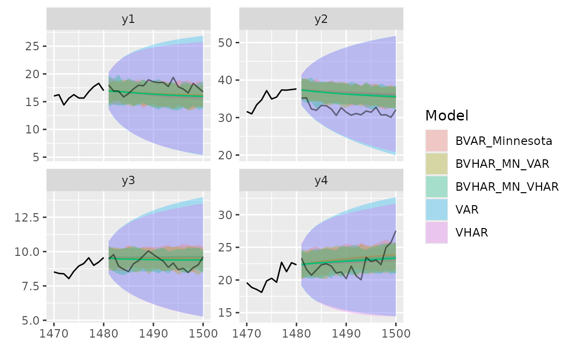
Error
Mean of MSE
list(
  VAR = mse_var,
  VHAR = mse_vhar,
  BVAR = mse_bvar,
  BVHAR1 = mse_bvhar_v1,
  BVHAR2 = mse_bvhar_v2
) |>
  lapply(mean) |>
  unlist() |>
  sort()
#>     VHAR      VAR   BVHAR1     BVAR   BVHAR2
#> 3.36e+00 3.36e+00 6.71e+20 2.82e+21 6.71e+36
For each variable, we can see the error with plot.
list(
  pred_var,
  pred_vhar,
  pred_bvar,
  pred_bvhar_v1,
  pred_bvhar_v2
) |>
  gg_loss(y = y_test, "mse")
#> Warning: `label` cannot be a <ggplot2::element_blank> object.
#> `label` cannot be a <ggplot2::element_blank> object.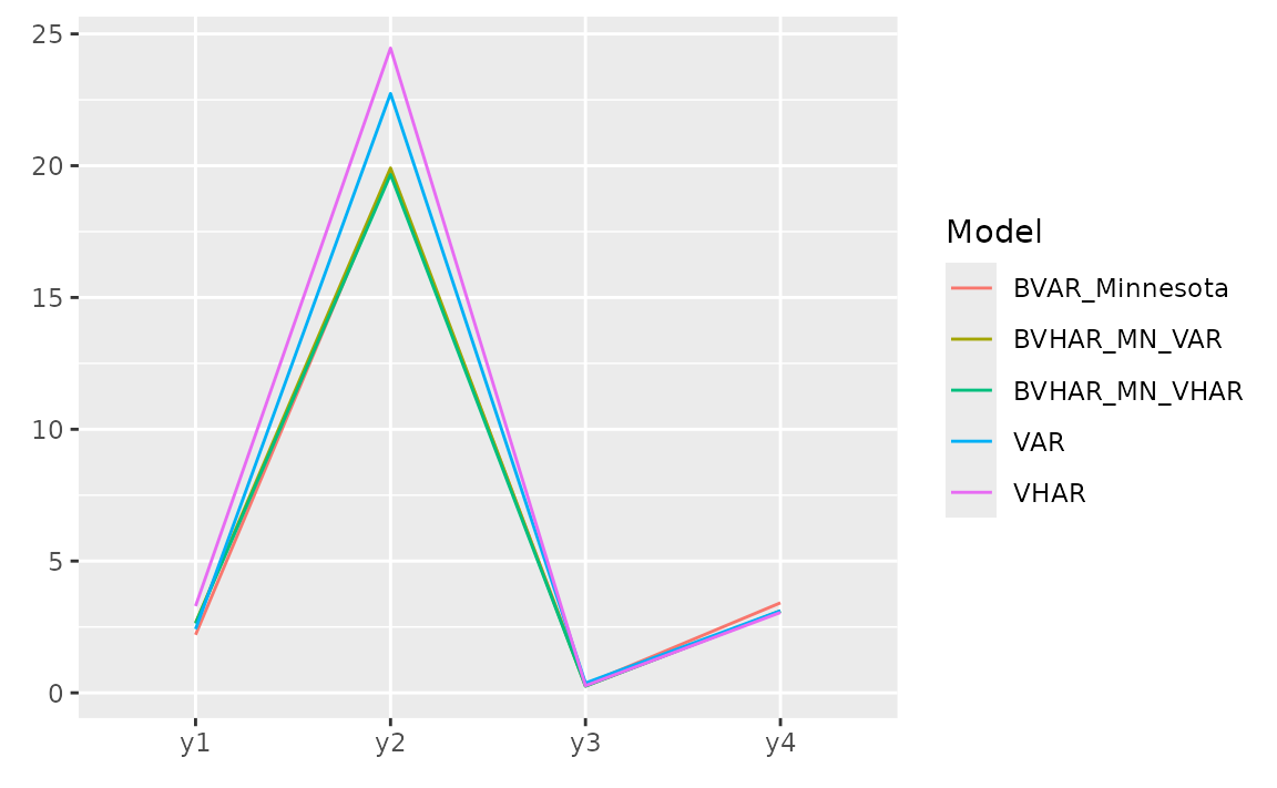
Relative MAPE (MAPE), benchmark model: VAR
Out-of-Sample Forecasting
In time series research, out-of-sample forecasting plays a key role. So, we provide out-of-sample forecasting function based on
- Rolling window:
forecast_roll(object, n_ahead, y_test) - Expanding window:
forecast_expand(object, n_ahead, y_test)
Rolling windows
forecast_roll(object, n_ahead, y_test) conducts h >=
1 step rolling windows forecasting.
It fixes window size and moves the window. The window is the training set. In this package, we set window size = original input data.
Iterating the step
- The model is fitted in the training set.
- With the fitted model, researcher should forecast the next h >= 1
step ahead. The longest forecast horizon is
num_test - h + 1. - After this window, move the window and do the same process.
- Get forecasted values until possible (longest forecast horizon).
5-step out-of-sample:
(var_roll <- forecast_roll(model_var, 5, y_test))
#>         y1   y2    y3   y4
#>  [1,] 19.7 26.0 10.58 32.3
#>  [2,] 18.6 25.1 10.08 31.3
#>  [3,] 18.4 24.3  9.84 30.9
#>  [4,] 18.1 24.5  9.68 30.5
#>  [5,] 19.2 25.5  9.99 31.3
#>  [6,] 19.2 26.8 10.23 30.9
#>  [7,] 19.3 27.3 10.13 30.1
#>  [8,] 20.4 28.2 10.38 29.5
#>  [9,] 20.1 28.3 10.30 30.3
#> [10,] 19.9 27.0 10.02 29.3
#> [11,] 19.6 26.7 10.05 29.5
#> [12,] 19.6 25.5  9.67 30.3
#> [13,] 20.8 26.6 10.14 29.8
#> [14,] 20.8 26.2 10.06 28.9
#> [15,] 20.6 25.6  9.91 28.9
#> [16,] 19.8 26.6 10.22 28.4
Denote that the nrow is longest forecast horizon.
class(var_roll)
#> [1] "predbvhar_roll" "bvharcv"
names(var_roll)
#> [1] "process"  "forecast" "eval_id"  "y"
To apply the same evaluation methods, a class named
bvharcv has been defined. You can use the functions
above.
vhar_roll <- forecast_roll(model_vhar, 5, y_test)
bvar_roll <- forecast_roll(model_bvar, 5, y_test)
bvhar_roll_v1 <- forecast_roll(model_bvhar_v1, 5, y_test)
bvhar_roll_v2 <- forecast_roll(model_bvhar_v2, 5, y_test)
Relative MAPE, benchmark model: VAR
Expanding Windows
forecast_expand(object, n_ahead, y_test) conducts h
>= 1 step expanding window forecasting.
Different with rolling windows, expanding windows method fixes the starting point. The other is same.
(var_expand <- forecast_expand(model_var, 5, y_test))
#>         y1   y2    y3   y4
#>  [1,] 19.7 26.0 10.58 32.3
#>  [2,] 18.6 25.1 10.09 31.3
#>  [3,] 18.4 24.4  9.84 30.9
#>  [4,] 18.1 24.5  9.68 30.4
#>  [5,] 19.2 25.6  9.99 31.3
#>  [6,] 19.2 26.8 10.25 30.9
#>  [7,] 19.3 27.3 10.15 30.2
#>  [8,] 20.4 28.2 10.39 29.6
#>  [9,] 20.0 28.3 10.31 30.3
#> [10,] 19.9 27.0 10.02 29.3
#> [11,] 19.6 26.7 10.06 29.5
#> [12,] 19.5 25.5  9.67 30.2
#> [13,] 20.7 26.6 10.13 29.8
#> [14,] 20.7 26.2 10.06 28.9
#> [15,] 20.5 25.6  9.92 28.9
#> [16,] 19.8 26.6 10.22 28.4
The class is bvharcv.
class(var_expand)
#> [1] "predbvhar_expand" "bvharcv"
names(var_expand)
#> [1] "process"  "forecast" "eval_id"  "y"
vhar_expand <- forecast_expand(model_vhar, 5, y_test)
bvar_expand <- forecast_expand(model_bvar, 5, y_test)
bvhar_expand_v1 <- forecast_expand(model_bvhar_v1, 5, y_test)
bvhar_expand_v2 <- forecast_expand(model_bvhar_v2, 5, y_test)
Relative MAPE, benchmark model: VAR