Bayesian VAR and VHAR Models • bvhar

library(bvhar)

etf <- etf_vix[1:55, 1:3]
# Split-------------------------------
h <- 5
etf_eval <- divide_ts(etf, h)
etf_train <- etf_eval$train
etf_test <- etf_eval$test

Bayesian VAR and VHAR

var_bayes() and vhar_bayes() fit BVAR and BVHAR each with various priors.

y: Multivariate time series data. It should be data frame or matrix, which means that every column is numeric. Each column indicates variable, i.e. it sould be wide format.
p or har: VAR lag, or order of VHAR
num_chains: Number of chains
- If OpenMP is enabled, parallel loop will be run.
num_iter: Total number of iterations
num_burn: Number of burn-in
thinning: Thinning
coef_spec: Coefficient prior specification.
- Minneosta prior
  - BVAR: set_bvar()
  - BVHAR: set_bvhar() and set_weight_bvhar()
  - Can induce prior on $\lambda$ using lambda = set_lambda()
- SSVS prior: set_ssvs()
- Horseshoe prior: set_horseshoe()
- NG prior: set_ng()
- DL prior: set_dl()
contem_spec: Contemporaneous prior specification.
cov_spec: Covariance prior specification. Use set_ldlt() for homoskedastic model.
include_mean = TRUE: By default, you include the constant term in the model.
minnesota = c("no", "short", "longrun"): Minnesota-type shrinkage.
verbose = FALSE: Progress bar
num_thread: Number of thread for OpenMP
- Used in parallel multi-chain loop
- This option is valid only when OpenMP in user’s machine.

Stochastic Search Variable Selection (SSVS) Prior

(fit_ssvs <- vhar_bayes(etf_train, num_chains = 1, num_iter = 20, coef_spec = set_ssvs(), contem_spec = set_ssvs(), cov_spec = set_ldlt(), include_mean = FALSE, minnesota = "longrun"))
#> Call:
#> vhar_bayes(y = etf_train, num_chains = 1, num_iter = 20, coef_spec = set_ssvs(), 
#>     contem_spec = set_ssvs(), cov_spec = set_ldlt(), include_mean = FALSE, 
#>     minnesota = "longrun")
#> 
#> BVHAR with SSVS prior + SSVS prior
#> Fitted by Gibbs sampling
#> Total number of iteration: 20
#> Number of burn-in: 10
#> ====================================================
#> 
#> Parameter Record:
#> # A draws_df: 10 iterations, 1 chains, and 90 variables
#>      phi[1]   phi[2]   phi[3]     phi[4]   phi[5]   phi[6]  phi[7]  phi[8]
#> 1   -0.0876  -0.0175  -0.2211   0.048667   0.2732   0.0339   0.755   0.355
#> 2    0.1705  -0.0185  -0.1899   0.198807  -0.0889  -0.0591  -0.169   0.201
#> 3   -0.1823  -0.3229  -0.1574  -0.000812   0.3271  -0.2168   0.614   0.154
#> 4   -0.0456   0.4376  -0.2301   0.105966  -0.7925  -0.1346  -0.401   0.235
#> 5    0.1391   0.5049  -0.3111  -0.383728  -0.7563  -0.1516   0.386   0.835
#> 6    0.1806  -0.1231   0.0320  -0.500005   0.1669  -0.4150   0.738   0.131
#> 7   -0.0620  -0.3463   0.1281  -0.177550   0.5410  -0.4273   1.408   0.466
#> 8    0.1520   0.3084  -0.0333  -0.851727  -0.5724  -0.4793   0.781   1.111
#> 9    0.2625  -0.0168  -0.0794  -0.864491   0.2769  -0.0485   0.494   0.621
#> 10   0.3484   0.5000  -0.2022  -0.970879  -0.5480  -0.1629   0.801   0.874
#> # ... with 82 more variables
#> # ... hidden reserved variables {'.chain', '.iteration', '.draw'}

autoplot() for the fit (bvharsp object) provides coefficients heatmap. There is type argument, and the default type = "coef" draws the heatmap.

autoplot(fit_ssvs)

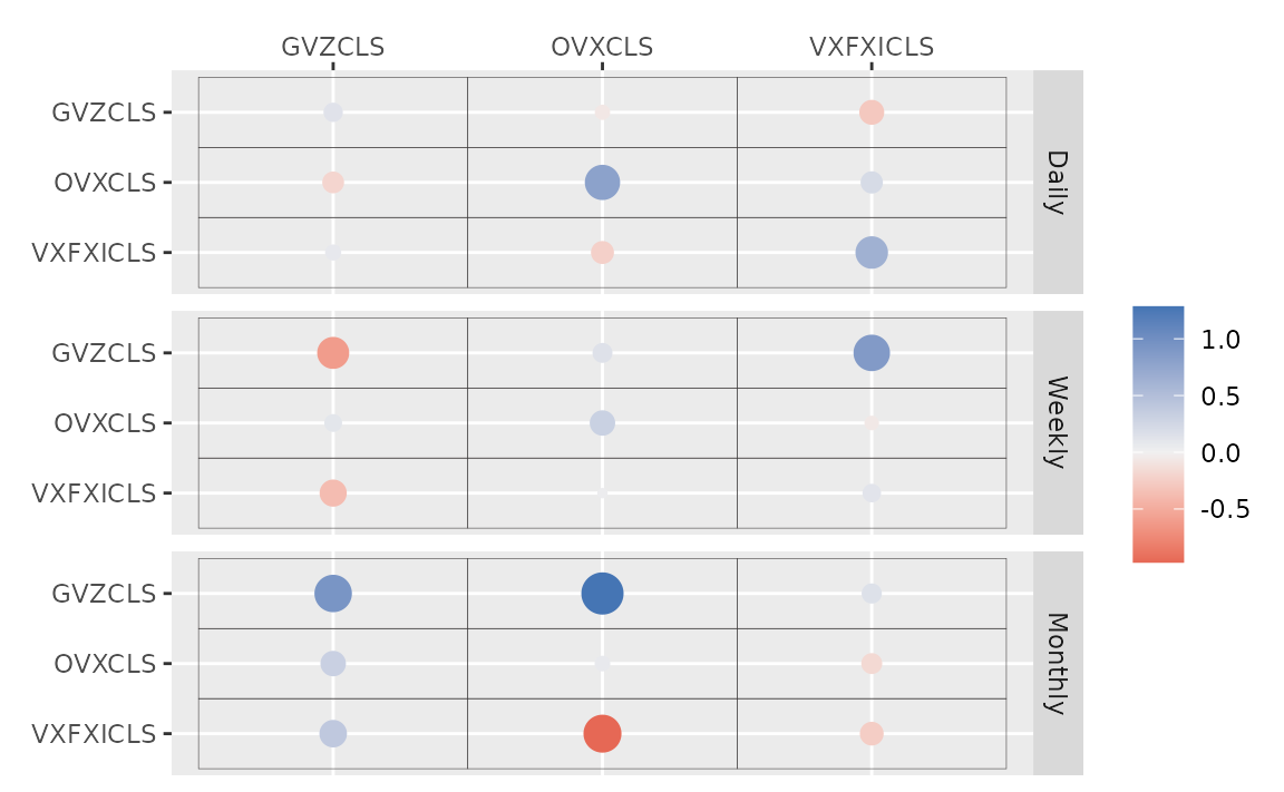
Horseshoe Prior

coef_spec is the initial specification by set_horseshoe(). Others are the same.

(fit_hs <- vhar_bayes(etf_train, num_chains = 2, num_iter = 20, coef_spec = set_horseshoe(), contem_spec = set_horseshoe(), cov_spec = set_ldlt(), include_mean = FALSE, minnesota = "longrun"))
#> Call:
#> vhar_bayes(y = etf_train, num_chains = 2, num_iter = 20, coef_spec = set_horseshoe(), 
#>     contem_spec = set_horseshoe(), cov_spec = set_ldlt(), include_mean = FALSE, 
#>     minnesota = "longrun")
#> 
#> BVHAR with Horseshoe prior + Horseshoe prior
#> Fitted by Gibbs sampling
#> Number of chains: 2
#> Total number of iteration: 20
#> Number of burn-in: 10
#> ====================================================
#> 
#> Parameter Record:
#> # A draws_df: 10 iterations, 2 chains, and 124 variables
#>       phi[1]   phi[2]     phi[3]   phi[4]  phi[5]  phi[6]     phi[7]   phi[8]
#> 1   -0.04495  -0.2428  -0.408630   0.2169   1.363   0.663  -2.49e-02  -0.1709
#> 2    0.08816   0.0361   0.000658  -0.2194   0.715   0.721   1.18e-02  -0.2143
#> 3    0.00684   0.0276  -0.111765   0.0407   1.079   0.931   3.58e-04  -0.0892
#> 4    0.00944   0.0530   0.168523  -0.0199  -0.477   0.959  -1.54e-03   0.0292
#> 5   -0.00226   0.0121  -0.054365   0.2389   0.682   0.971   1.99e-03   0.0678
#> 6    0.03164  -0.0434  -0.105660  -0.0190   0.203   0.898   2.89e-04   0.0595
#> 7   -0.20536  -0.1265  -0.009287   0.4954  -0.123   0.608   1.29e-04  -0.1439
#> 8    0.00274  -0.1432  -0.000363  -0.1834   0.194   0.679  -6.89e-05  -0.1870
#> 9    0.16452  -0.0938   0.009767  -0.0540   0.255   0.573  -5.64e-04  -0.2881
#> 10   0.18610  -0.3555   0.000239   0.4681  -0.181   0.686   1.01e-03  -0.2060
#> # ... with 10 more draws, and 116 more variables
#> # ... hidden reserved variables {'.chain', '.iteration', '.draw'}

autoplot(fit_hs)

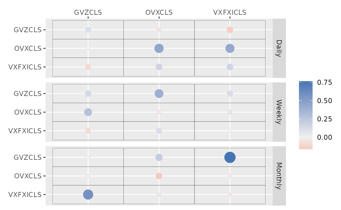
Minnesota Prior

(fit_mn <- vhar_bayes(etf_train, num_chains = 2, num_iter = 20, coef_spec = set_bvhar(lambda = set_lambda()), cov_spec = set_ldlt(), include_mean = FALSE, minnesota = "longrun"))
#> Call:
#> vhar_bayes(y = etf_train, num_chains = 2, num_iter = 20, coef_spec = set_bvhar(lambda = set_lambda()), 
#>     cov_spec = set_ldlt(), include_mean = FALSE, minnesota = "longrun")
#> 
#> BVHAR with MN_Hierarchical prior + MN_Hierarchical prior
#> Fitted by Gibbs sampling
#> Number of chains: 2
#> Total number of iteration: 20
#> Number of burn-in: 10
#> ====================================================
#> 
#> Parameter Record:
#> # A draws_df: 10 iterations, 2 chains, and 63 variables
#>      phi[1]    phi[2]    phi[3]    phi[4]    phi[5]  phi[6]   phi[7]   phi[8]
#> 1    0.0772  -0.19792  -0.02059   0.02107   0.18810   0.653   0.6363  -0.1294
#> 2    0.1971   0.03031   0.02267  -0.16524   0.16601   0.963   0.5907   0.1467
#> 3   -0.0652   0.04858   0.13853   0.41502   0.21091   0.913   0.0569  -0.2873
#> 4    0.0462   0.01200   0.24799   0.28023   0.05044   1.155  -0.0932   0.0422
#> 5    0.3616  -0.13088   0.16699   0.00432   0.12119   0.705  -0.0217   0.1122
#> 6    0.3236  -0.11465   0.01582   0.03471   0.00207   0.675  -0.1075  -0.0457
#> 7    0.1022  -0.11147  -0.00271  -0.00526   0.11684   0.538   0.3197   0.0984
#> 8    0.2079   0.00524   0.02906  -0.06189  -0.07685   0.781   0.1671   0.0594
#> 9    0.4017  -0.11320   0.07950  -0.08998   0.05990   0.959   0.2355  -0.1646
#> 10   0.2470  -0.29699   0.25608  -0.05925  -0.00420   0.736   0.2196  -0.2519
#> # ... with 10 more draws, and 55 more variables
#> # ... hidden reserved variables {'.chain', '.iteration', '.draw'}

Normal-Gamma prior

(fit_ng <- vhar_bayes(etf_train, num_chains = 2, num_iter = 20, coef_spec = set_ng(), cov_spec = set_ldlt(), include_mean = FALSE, minnesota = "longrun"))
#> Call:
#> vhar_bayes(y = etf_train, num_chains = 2, num_iter = 20, coef_spec = set_ng(), 
#>     cov_spec = set_ldlt(), include_mean = FALSE, minnesota = "longrun")
#> 
#> BVHAR with NG prior + NG prior
#> Fitted by Metropolis-within-Gibbs
#> Number of chains: 2
#> Total number of iteration: 20
#> Number of burn-in: 10
#> ====================================================
#> 
#> Parameter Record:
#> # A draws_df: 10 iterations, 2 chains, and 97 variables
#>       phi[1]    phi[2]    phi[3]    phi[4]   phi[5]  phi[6]    phi[7]   phi[8]
#> 1    0.29085   0.01876   0.00254   0.53359   0.7936   1.001  -0.00506  -0.1146
#> 2    0.27410  -0.00536  -0.00289  -0.08364   0.3323   0.916   0.00200   0.0479
#> 3    0.14191   0.00524  -0.00385   0.04266   0.5909   1.105   0.24897  -0.0465
#> 4    0.14230  -0.00688  -0.00775  -0.08325   0.2356   1.178  -0.06971  -0.0873
#> 5    0.06147  -0.08083  -0.01876  -0.01126   0.3633   0.905   0.01817  -0.0240
#> 6    0.01886   0.10961  -0.01871  -0.01531   0.0815   1.002   0.01369   0.0155
#> 7    0.06842  -0.01518  -0.04223   0.03511  -0.0854   1.007  -0.05042   0.0542
#> 8    0.10784  -0.00400  -0.02816  -0.00807  -0.1218   0.967  -0.04223  -0.0218
#> 9   -0.00779  -0.04138   0.03443  -0.00719  -0.0669   0.914  -0.02592   0.0282
#> 10  -0.05957  -0.04837   0.03679  -0.05329  -0.4538   0.989   0.49214   0.0819
#> # ... with 10 more draws, and 89 more variables
#> # ... hidden reserved variables {'.chain', '.iteration', '.draw'}

Dirichlet-Laplace prior

(fit_dl <- vhar_bayes(etf_train, num_chains = 2, num_iter = 20, coef_spec = set_dl(), cov_spec = set_ldlt(), include_mean = FALSE, minnesota = "longrun"))
#> Call:
#> vhar_bayes(y = etf_train, num_chains = 2, num_iter = 20, coef_spec = set_dl(), 
#>     cov_spec = set_ldlt(), include_mean = FALSE, minnesota = "longrun")
#> 
#> BVHAR with DL prior + DL prior
#> Fitted by Gibbs sampling
#> Number of chains: 2
#> Total number of iteration: 20
#> Number of burn-in: 10
#> ====================================================
#> 
#> Parameter Record:
#> # A draws_df: 10 iterations, 2 chains, and 91 variables
#>      phi[1]    phi[2]     phi[3]    phi[4]    phi[5]  phi[6]    phi[7]
#> 1    0.6649  -0.01237   0.069009   0.00561   0.00749   0.887  0.009225
#> 2   -0.1599   0.01815  -0.028959  -0.19610   0.00201   1.001  0.001811
#> 3    0.0283   0.03827   0.005455  -0.09079  -0.02481   0.657  0.000324
#> 4   -0.0746   0.00349  -0.002459  -0.10138  -0.02564   0.832  0.000957
#> 5   -0.0768   0.00363   0.000592  -0.20245  -0.00701   0.787  0.004184
#> 6    0.0236  -0.00258   0.000969   0.22434   0.00141   0.895  0.005828
#> 7    0.0999   0.00342   0.002082  -0.16765  -0.00407   0.934  0.001044
#> 8    0.0550  -0.02013  -0.005254  -0.05116   0.00145   0.852  0.000293
#> 9    0.1261   0.00336   0.001000   0.08824   0.00059   0.878  0.000241
#> 10   0.0254   0.00176   0.000370  -0.02905   0.02248   0.923  0.000737
#>        phi[8]
#> 1   -8.08e-02
#> 2   -2.20e-02
#> 3   -2.42e-02
#> 4   -8.51e-04
#> 5    2.29e-04
#> 6   -1.89e-05
#> 7   -2.54e-04
#> 8   -1.57e-04
#> 9    5.62e-04
#> 10  -5.38e-04
#> # ... with 10 more draws, and 83 more variables
#> # ... hidden reserved variables {'.chain', '.iteration', '.draw'}

Bayesian visualization

autoplot() also provides Bayesian visualization. type = "trace" gives MCMC trace plot.

autoplot(fit_hs, type = "trace", regex_pars = "tau")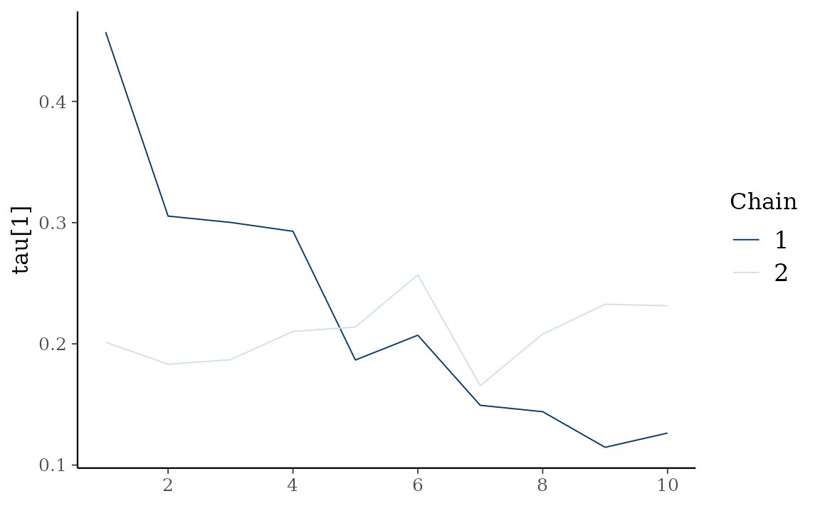

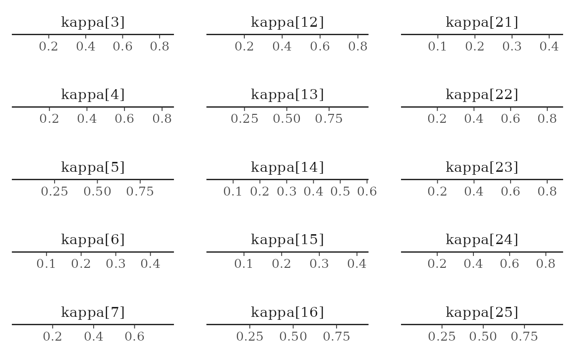
type = "dens" draws MCMC density plot. If specifying additional argument facet_args = list(dir = "v") of bayesplot, you can see plot as the same format with coefficient matrix.

autoplot(fit_hs, type = "dens", regex_pars = "kappa", facet_args = list(dir = "v", nrow = nrow(fit_hs$coefficients)))